Artificial Intelligence, Deep learning and Neural nets are all buzzwords these days and it can be quite intimidating given the rapid growth and interest in the area. I am going to solve this in two code dumps (one if you are in a hurry). Because you are already here, I am going to assume you don't need any convincing of the vast potential of Neural Networks, but if you do - click the top title to jump to my home page where there are lots of articles I have written on the merits of Neural Nets.

If you stick with me for the first code dump (30 lines) you will understand the core concept of how a Neural Network is used to build predictive models. If you are still around near halfway down the page for the second code dump (50 ~ lines) then you will see the hidden sauce which makes DeepLearning and Neural networks the hype they are today - backwards propagation.

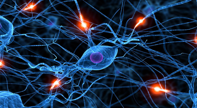
Neural Networks exist both in nature (the structure of neurons in your brain) and in software - the digital imitation of this process

All the code here is in Python, I suggest you use an IDE like pycharm but if you are up for learning new things then Jupyter notebook is the way to go (it's what I wrote this blog in).

The image below shows a list of input/output relationships.
In the source code below, we are going to try and predict the output values by allowing the network to tune itself in the direction of the actual output so that the NN arrives at the answer independently. What we have in the end is a tuned 'model'.
Imagine you are trying to predict the output given the inputs, in this case there is a perfect correlation.

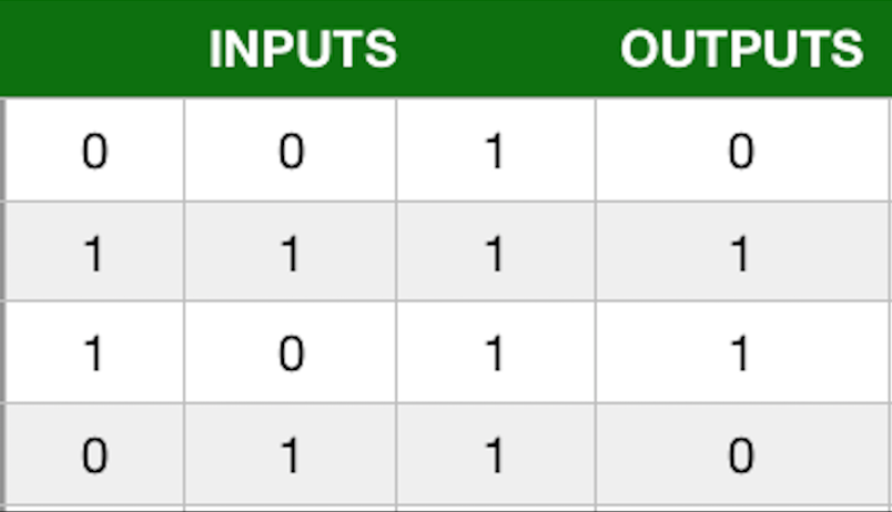
Above is a table of input output parameters. You can think of this as each row being a training case for the network, where it has to work out the output given a set of inputs

Models are necessery for applications in real life, for example, if this was a fraud engine the model would give us a probability of fraud given certain input parameters. In this case, the outputs 1 would be fraud and 0 would be instances of no fraud. Of course this model would be far too simple, but the basic principles are the same.

Lets go straight to the code, I will explain the key steps afterwards. This network performs forward propagation, basically there are two layers at each layer calculations are performed on nodes to steer in the direction of desired values.

import numpy as np


#SIGMOID FUNCTION 
def sigmoid(x,deriv=False): # deriv is a trigger we set based upon the function boolean passed in 
    if(deriv==True):
        return x*(1-x)
    return 1/(1+np.exp(-x))

X = np.array([  [0,0,1],
                [1,1,1],
                [1,0,1],
                [0,1,1] ])


y = np.array([[0,1,1,0]]).T # TRANSPOSE IT  

# seed random numbers to make calculation
# deterministic (just a good practice)
np.random.seed(1)

syn0 = 2*np.random.random((3,1)) - 1    #synaptic weigths 


for iter in range(10000):
    
    
    #forward propagate
    l0 = X
    l1 = sigmoid(np.dot(l0,syn0))

    
    #how much did we miss by? 
    l1_error = y - l1
    
    
    
    # MULTIPLY THE AMOUNT WE MISSED BY THE
    # SLOPE OF THE SIGMOID AT THE VALUES IN L1
    l1_delta = l1_error * sigmoid(l1,True)
    
    
    #update weights 
    syn0 += np.dot(l0.T,l1_delta)
    
    
print("training complete")
print(l1)

training complete
[[ 0.00966449]
 [ 0.99211957]
 [ 0.99358898]
 [ 0.00786506]]

We did it!

If you round these numbers, you get 0,1,1,0 - basically our network has converged statistically to the correct answers. It will never reach 1 nor 0, but the distinction is so obvious that in practice there is no difference.

Below is a quick break down of some of the variables used,further down is a more definitive description of what just happened lol.

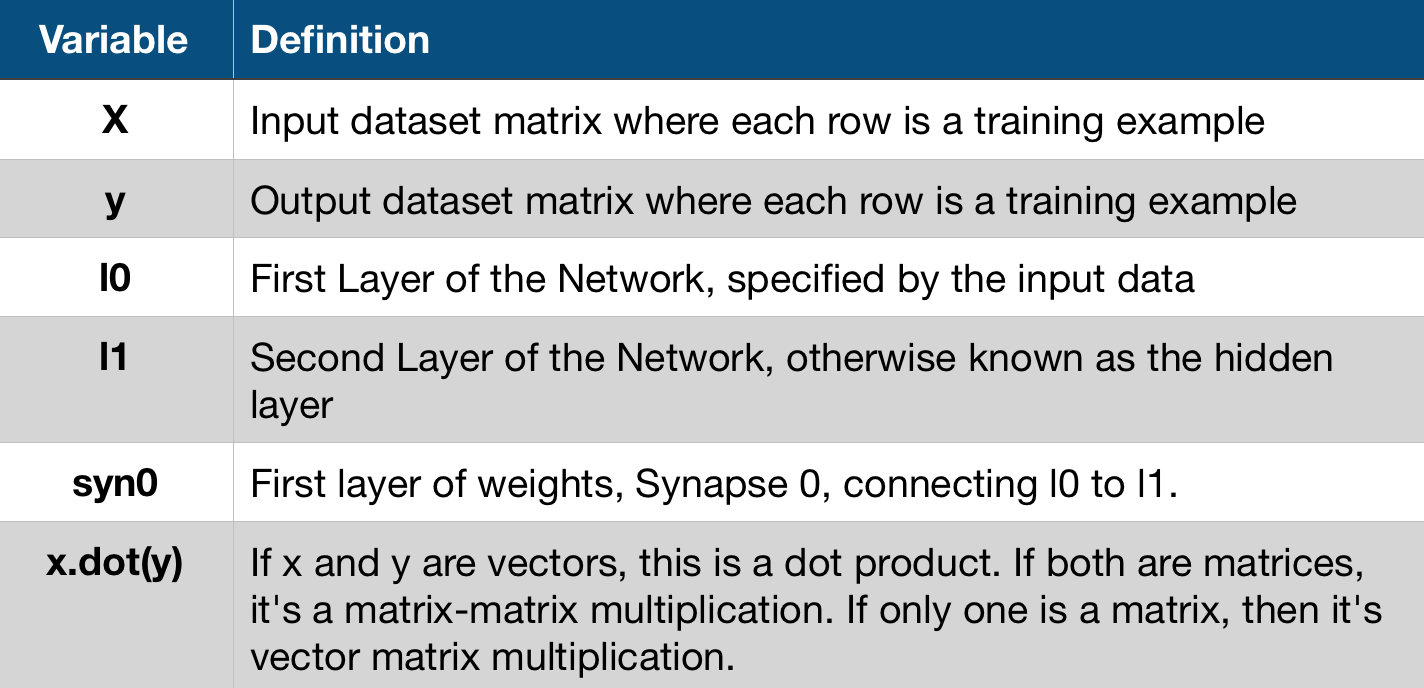
Above is a brief breakdown of some of the variables and functions used, I will give more details below.

1. Our network ran 10000 times
2. Each time L1 got closer and closer to the predicted values (try printing l1 in the loop)
3. The most important part is l1_delta = l1_error * nonlin(l1,True), this is slope of sigmoid more on this in another blog, but the bigger the slope the more certain the prediction.
4. This part (syn0 += np.dot(l0.T,l1_delta)) of the code is the actual end game, it is where we update our weights i.e. this is building our model. In the future if applied in a real life context, it would be the part that takes any input you give it and predict an output

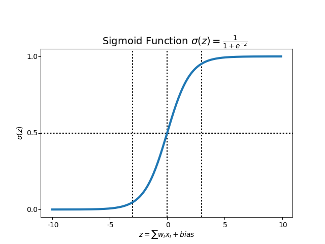
^^ that's it (don't worry if you don't get it)

Remember the bit in our code which said sigmoid? It was a non linear function, and does pretty much what the graph shows you above, it maps any of our numbers to a range between -1 and 1 i.e. 90 might be 0.87 and 12 might be 0.14. This allows us to convert numbers to probabilities.

Without going into to much detail, for our l1 we apply the sigmoid for probabilities but later we need to work out how much our error is (that is the slope of the graph). If you remember from calculus classes, to work out the slope you need to take the derrivative (hence how our funcion also can return the derivitive if we ask it to) and indeed we do when we work out the l1_delta.

By seeding the numbers we get a random distribution, but each time round they are randomly distributed in the same way each time we train the network. This makes it easier for us to see how our changes impact on the network.

In neuroscience and computer science, synaptic weight refers to the strength or amplitude of a connection between two nodes, corresponding in biology to the amount of influence the firing of one neuron has on another.

In our code this is quite analogous, this is our weight matrix for our neural network that we called syn0. Basically it is saying it is the zeroth synapse, if we had more layers we would have more synapses (like we do in the second part of this tutorial with syn0 and syn1for our three layer network).

To break it down a bit more, we made only two layers (input and output) so we need only one matrix of weights to connect them. That matrix is size (3,1) because we have three inputs and one outputs. It needs to multiply each value by a certain amount so needs to connect to each one, hence the size (3,1).

Since we have size L0 = 3 and size L1 = 1 so we need shape syn0 = (3,1)

Some final points, we initialize syn0 randomly, and it should get updated over time - because this is where the learning is stored, not in the input output X, Y values.

As you may have guessed the actually training happens within the loop, L0 = X because it is the first layer, remember that X has four input values(rows) but we process them at the same time. This is called full batch training, you don't need to know anything else other than more complex models break it down at row level.

l1 = nonlin(np.dot(l0,syn0)) is our step where we perform predictions. Basically we take a stab then adjust each iteration. The equation takes the dot product of l0 and syn0 (in this case multiplies them) then passes the result through the sigmoid function. This is a bit complicated and i definitely recommend more study as you go, but for now this is a matrix multiplication of layer0 (i.e. input) by our weights.

Our value l1 represents a 'stab' at each of our inputs, we now subtract the actual output value (y) from this guess. The results is either positive or negative, i.e. the difference represents how much we missed by for our four inputs and represented as a vector.

This is quite tough to grasp without a background in calculus, I will explain the basic principle here then go into more detail at the end in the theory section (that may be a work in progress). Generally we want to preserve the state of high confidence predictions and banish the low confidence guesses. This is what multiplying the slope by the error does.

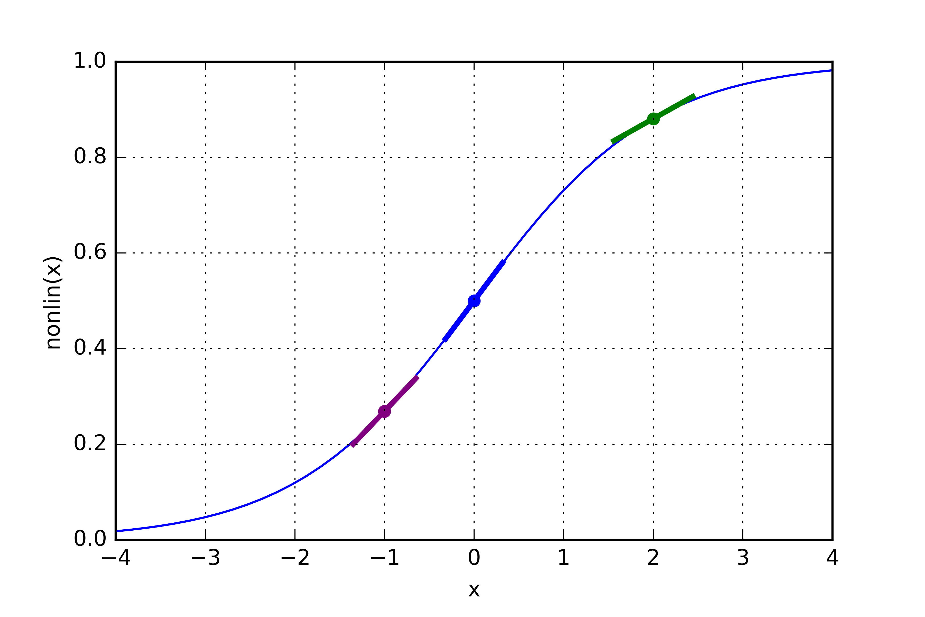
If you look at the sigma graph, any value on the curve that is close to Y = 1 or Y = 0 will have a shallow slope. The slope is at the steepest in the middle, (in fact taking the slope of the sigma curve is what differentiating means).
So in our code we have l1_delta = l1_error * nonlin(l1,True) and l2_delta = l2_error * nonlin(l2,True), in both of these cases we are saying, if the curve is shallow, then the number will be close to 0 and thus the delta will be small. The end game is to reduce the detla, so the model is as accurate as possible. The final step where we update our weights, is the learning process and this of course involves replicating delta!!

aaaaaaaand we are done!

Ok, that was a lot to take in! For now read over the notes a few times until you are comfortable. If you got this far, seriously a huge well done - you have built your first network that statistically converges on the right model - independently, pretty neat eh? This is what machine learning is all about! Next week I will pick up on a three layer neural network (with the magic sauce - back propagation).
Many thanks for reading, please like or share below if you want to see more.

Adam McMurchie

06/June/2018